Phillips Curve explained: inflation, unemployment and the limits of monetary policy

What is the Phillips Curve?

The Phillips Curve was introduced in 1958 by A.W. Phillips, who studied the relationship between unemployment and wage inflation in the United Kingdom. His research found that wage growth generally accelerated when unemployment was low and weakened when unemployment was high.

The underlying mechanism begins with the labour market

When businesses compete for a limited pool of available workers, they may offer higher wages to attract and retain employees. Rising labour costs can put pressure on company margins, while stronger household incomes can support consumer spending. If demand is strong enough, businesses may pass higher costs on to customers.

When unemployment rises, workers generally have less bargaining power and businesses face less pressure to increase wages. If consumer demand also weakens, companies may find it harder to raise prices.

The traditional Phillips Curve therefore suggests an inverse relationship between unemployment and inflation. However, it describes a tendency, not a rule. Inflation can rise even when unemployment is high if energy prices surge, supply chains deteriorate or inflation expectations increase.

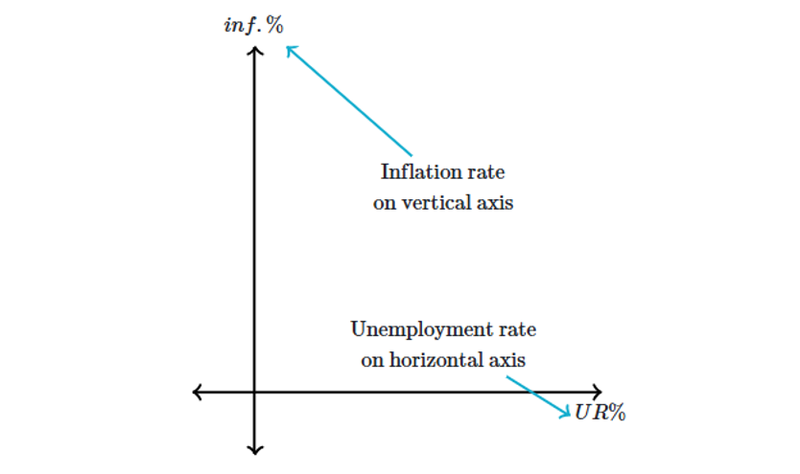
Source: Khan academy

Short-run vs. long-run Phillips Curve

The Short-Run Phillips Curve (SRPC) slopes downward, illustrating a potential trade-off between inflation and unemployment. In the short run, expansionary monetary or fiscal policy can stimulate aggregate demand, encourage hiring and reduce unemployment, but it can also increase inflationary pressure.

If demand grows faster than the economy's productive capacity, businesses may raise prices and workers may demand higher wages. Inflation can accelerate as the labour market tightens.

The reverse can happen when interest rates rise. Higher borrowing costs can slow consumption and investment, weaken demand for workers and reduce inflationary pressure, although employment may also suffer.

The long-run Phillips Curve

The Long-Run Phillips Curve (LRPC) is traditionally represented as a vertical line at the natural rate of unemployment. This reflects the argument that policymakers cannot permanently reduce unemployment below its sustainable level simply by accepting higher inflation.

The Non-Accelerating Inflation Rate of Unemployment, or NAIRU, is an estimate of the unemployment rate consistent with inflation that is not persistently accelerating. It is closely related to the natural rate of unemployment, although the concepts are not identical in every economic framework.

The adjustment occurs through expectations. If workers and businesses begin to expect higher inflation, employees may demand larger wage increases and companies may raise prices in anticipation of higher costs. The short-run Phillips Curve can shift upward, leaving the economy with higher inflation even if unemployment returns to its sustainable level.

Example of Phillips Curve

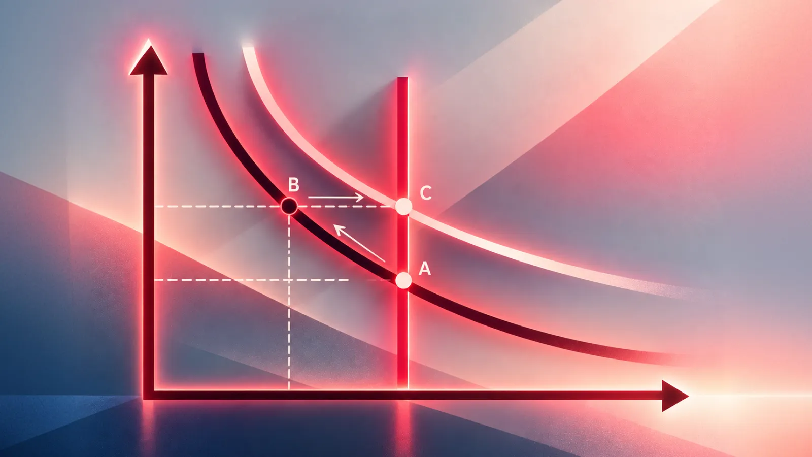
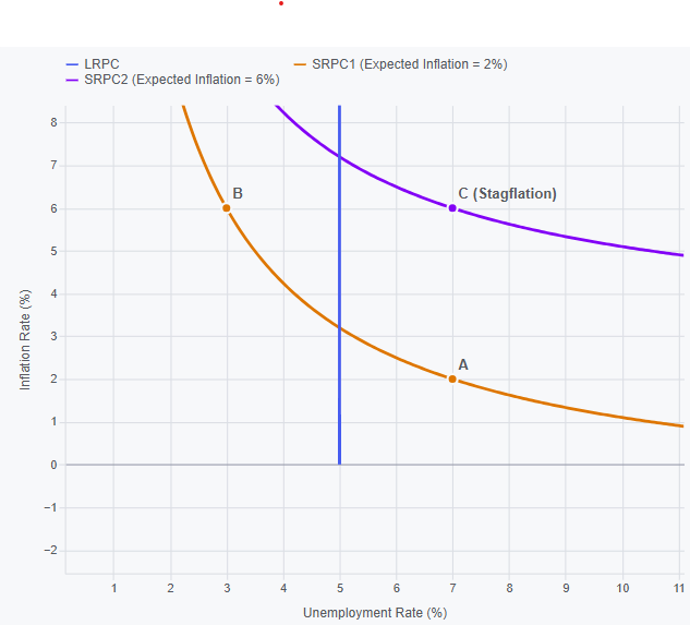
On the original short-run Phillips Curve (SRPC1), Point A represents a period of relatively low inflation and high unemployment, typically associated with weak aggregate demand and limited pressure on prices.

Point B shows the opposite situation, where stronger demand reduces unemployment but pushes inflation higher as businesses compete for workers and raise prices.

Point C demonstrates stagflation, where inflation and unemployment are both high. Unlike the movement between Points A and B, this outcome reflects a shift in the short-run Phillips Curve from SRPC1 to SRPC2, driven by higher expected inflation or an adverse supply shock.

The oil crises of the 1970s provide a historical example, as surging energy costs pushed prices higher while weakening economic activity and increasing unemployment. The key lesson is that the trade-off between inflation and unemployment is not fixed.

When inflation expectations change or production costs rise sharply, the entire curve can shift, leaving policymakers facing higher inflation and weaker employment at the same time.

Source: ChatGPT – authors idea

The great inflation era: United States, 1964–1980

Great Inflation provides one of the clearest historical demonstrations of why the short-run trade-off cannot be treated as permanent.

During the 1960s, expansionary fiscal policy supported spending through programmes associated with the Vietnam War and President Lyndon Johnson's Great Society. Monetary policy also accommodated strong demand during parts of the period.

The labour market tightened considerably

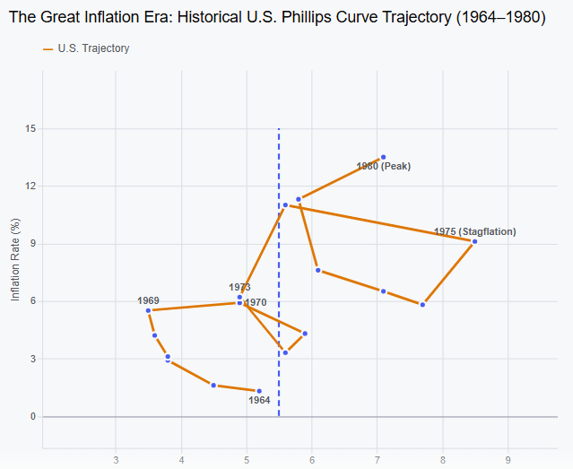
Unemployment fell from approximately 5.2% in 1964 to around 3.5% in 1969, while inflation accelerated from low levels to considerably higher rates. The initial pattern appeared consistent with the short-run Phillips Curve: stronger demand and lower unemployment coincided with rising inflation.

But the inflationary pressure did not disappear when the economy moved into the 1970s. Workers and businesses increasingly had to account for higher expected inflation in wage negotiations and pricing decisions. Once inflation expectations became embedded, bringing inflation down became more difficult.

The historical data show how sharply the environment deteriorated

By 1974, U.S. inflation was around 11% on an annual-average CPI basis, while unemployment averaged approximately 5.6%. By 1980, inflation had reached around 13.5% and unemployment averaged approximately 7.1%.

What caused the breakdown?

The oil shocks of the 1970s were central to the deterioration. The 1973 oil embargo disrupted supplies and contributed to a sharp increase in energy prices. A second major oil shock followed in 1979, associated with the Iranian Revolution and disruptions to oil production and exports.

Higher oil prices increased transportation, manufacturing and production costs. Businesses faced more expensive inputs, while households had less purchasing power available for other goods and services. Economic activity weakened even as prices continued to rise.

Source: ChatGPT- Authors’ idea

Supply shocks: Why the entire curve can shift

A supply shock changes the cost or availability of goods and services. An adverse shock, such as a sharp increase in oil prices, can push inflation higher even when unemployment is rising and demand is weakening.

This is different from moving along an unchanged short-run Phillips Curve. At a given unemployment rate, inflation may now be higher than before because businesses face greater production costs.

Inflation expectations can make the effect more persistent

If workers expect prices to continue rising, they may demand higher wages. Companies may then increase prices to offset labour costs, spreading the initial shock across the economy.

Favourable supply developments can have the opposite effect. Lower energy prices, improved supply chains or stronger productivity can reduce production costs and ease inflation without requiring a substantial increase in unemployment.

For central banks, the source of inflation therefore matters. Higher interest rates can reduce demand, but they cannot directly restore disrupted oil production or remove a physical shortage of goods. Policymakers must assess whether a supply shock is temporary or likely to become embedded in wages and prices.

The U.S. economic expansion: 2015–2019

The expansion between 2015 and 2019 offers a contrasting example. The labour market strengthened substantially, yet inflation remained relatively subdued compared with the experience of the 1970s.

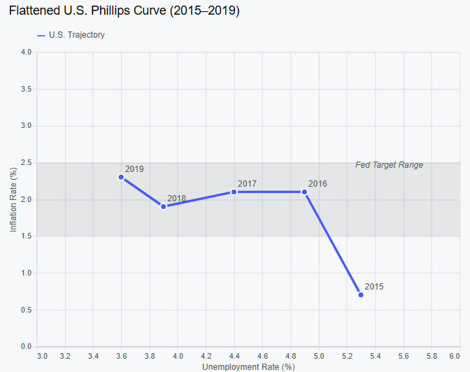
U.S. unemployment averaged approximately 5.3% in 2015 and reached 3.5% in late 2019, its lowest level in roughly half a century. Economic growth continued, borrowing costs remained relatively low for much of the period and employers increasingly competed for workers.

Under the simplest Phillips Curve interpretation, such a tight labour market should have generated a much larger increase in inflation. Instead, inflation remained close to the Federal Reserve's 2% objective for much of the expansion, depending on the measure used.

This episode suggested that the short-run Phillips Curve had become flatter. Falling unemployment did not produce the same degree of inflationary pressure that earlier economic models might have predicted.

Several factors help explain the difference

Inflation expectations were relatively well anchored, reducing the likelihood that moderate wage increases would trigger a persistent price-wage spiral. Global competition, productivity developments and changes in the labour market also limited the extent to which tighter employment conditions translated into consumer prices.

Fed Chair Jerome Powell highlighted this puzzle in 2018, noting that inflation had remained low despite a substantial improvement in labour-market conditions. The relationship remained relevant, but it had become weaker and more difficult to estimate.

The lesson is not that low unemployment no longer matters for inflation. Rather, the relationship depends on the wider economic environment. A tight labour market may generate only modest price pressure when expectations remain stable, and businesses can absorb higher costs or meet demand without substantial price increases.

Source: ChatGPT- Authors’ idea

The post-lockdown reopening: 2021

The U.S. recovery from the pandemic provides a more complicated example of rising demand meeting constrained supply.

In January 2021, unemployment stood at approximately 6.4%, while annual headline CPI inflation was 1.4%. By December, unemployment had fallen to 3.9%, and headline CPI inflation had climbed to 7.0%.

The initial recovery brought together several forces. Government stimulus supported household finances, vaccines enabled more economic activity and consumers began spending on goods and services that had been restricted during lockdowns.

Demand recovered quickly, but supply could not adjust at the same pace. Businesses faced labour shortages, transportation bottlenecks, shortages of materials and difficulties rebuilding inventories. Demand for goods was particularly strong, placing pressure on production and shipping networks.

The result was not a pure demand-pull episode

Strong spending helped drive inflation, but supply constraints were already contributing to price increases during 2021. Energy and food pressures subsequently intensified, while Russia's invasion of Ukraine in 2022 added further pressure to global commodity markets.

This distinction matters when interpreting Phillips Curve

Falling unemployment and accelerating inflation were consistent with a tightening labour market, but the scale of the inflation surge cannot be explained by unemployment alone.

The reopening demonstrated how demand pressures and supply disruptions can reinforce one another. It also showed why central banks need to distinguish between inflation caused by excessive spending and inflation caused by shortages or rising input costs.

Why the Phillips Curve matters for central banks

When unemployment is low, wage growth is accelerating and services inflation remains persistent, policymakers may conclude that demand is running ahead of the economy's capacity. This can support expectations for higher interest rates or a longer period of restrictive monetary policy.

When unemployment rises, hiring weakens and wage growth moderates, inflationary pressure may ease. That can give policymakers more room to lower interest rates, provided inflation expectations remain under control.

But the conclusion changes when a supply shock occurs

A surge in oil prices can lift headline inflation even as the labour market weakens. In that situation, central banks must judge whether the shock will fade or spread into wages, services and broader inflation expectations.

These distinctions matter to financial markets

Changes in expected interest rates can influence Treasury yields, the U.S. dollar and equity valuations. A cooling labour market alongside falling inflation may support expectations for monetary easing, while stagflation can create a more difficult environment because inflation remains high as economic growth deteriorates.